Hidden Markov Models (HMM)
Hidden Markov Models (HMM)
Go home
According to Dan Jurafsky and James Martin’s book Speech and Language Processing, a hidden markov model (HMM) is comprised of the following 5 components:
- Q: a set of N states.
- A: a transition probability matrix, with each element aij representing the probability of transitioning from state i to state j, subject to the constraint that the sum of these elements is 1 (forming a proper probability distribution)
- O: a set of T observations, each one drawn from a vocabulary V.
- B: a set of observation likelihoods, also called emission probabilities, each expressing the probability of an observation ot being generated from a state i.
- pi: an initial probability distribution over states. pi i is the probability that the markov chain will start in state i. Some states j may have pi j = 0, meaning they cannot be initial states. As with the transition probabilities, all must sum to one to form a valid probability distribution.
A first-order hidden Markov model instantiates two simplifying assumptions:
- First, as with a first-order Markov chain, the probability of a particular state depends only on the previous state: Markov Assumption:
- Second, the probability of an output observation oi depends only on the state that produced the observation qi and not on any other states or any other observations: Output Independence:
An HMM has two probability matrices, A and B:
- Matrix A contains the tag transition probabilities P(ti given ti−1) which represent the probability of a tag occurring given the previous tag. We compute the maximum likelihood estimate of this transition probability by counting, out of the times we see the first tag in a labeled corpus, how often the first tag is followed by the second:
- This matrix will have dimensions (N * N), where N is the number of tags.
- Matrix B (emission probabilities, P(wi given ti)), represents the probability, given a tag, that it will be associated with a given word. The MLE of the emission probability is:
The goal of HMM decoding:
- Given an HMM λ = (A,B), and a sequence of observations O, find the most probable sequence of states Q:
- The way we would do this in the context of an HMM is to use Bayes’ rule:
- We can simplify a bit by dropping the denominator:
HMM taggers make two further simplifying assumptions:
- The first is that the probability of a word appearing depends only on its own tag and is independent of neighboring words and tags:
- The second assumption, the bigram assumption, is that the probability of a tag is dependent only on the previous tag, rather than the entire tag sequence:
With our two simplifying assumptions, the equation for the most probable tag sequence simplifies to:
Corresponds to our emission probability matrix.
Corresponds to our transmission probability matrix.
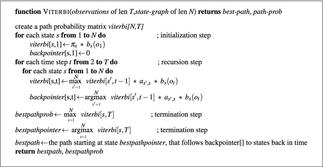
The Viterbi decoding algorithm:
- First, set up a probability matrix (or lattice), with one column for each observation ot and one row for each state in the state graph.
- Each cell of the trellis, vt(j), represents the probability that the HMM is in state j after seeing the first t observations and passing through the most probable state sequence q1,…,qt−1, given the HMM λ.
- The value of each cell vt(j) is computed by recursively taking the most probable path that could lead us to this cell.
- Formally, each cell expresses the probability vt(j):
- We represent the most probable path by taking the maximum over all possible previous state sequences max q1,…,qt−1
